Search Blogs

Showing results for "Prefix Sum"

Found 7 results

Equilibrium Point

Equilibrium Point

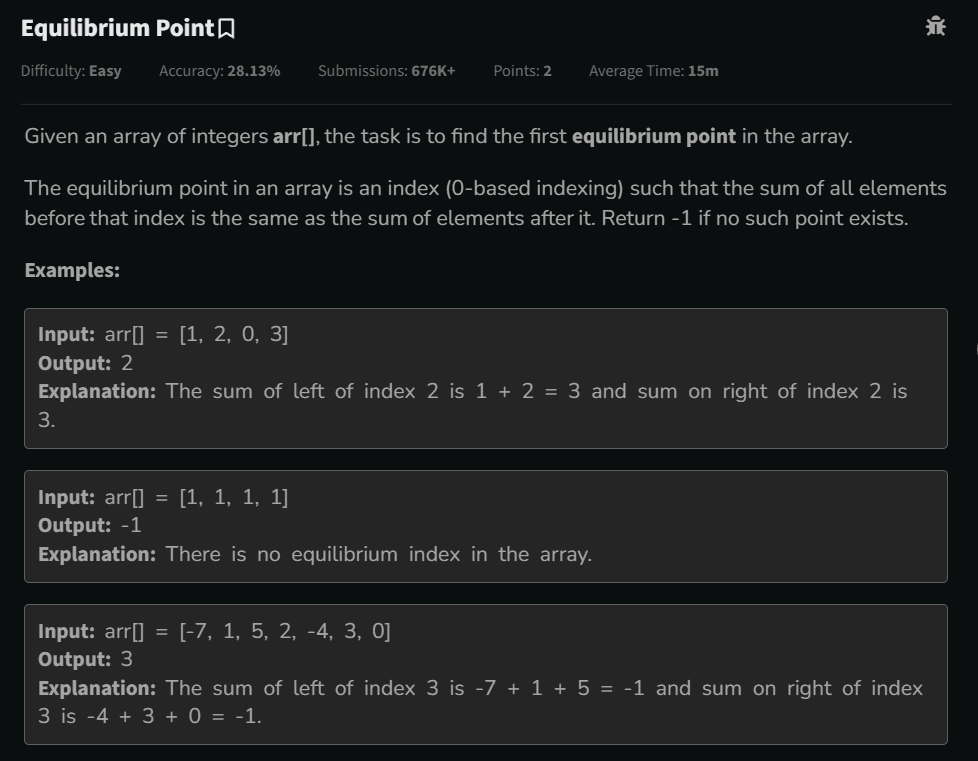
GeeksforGeeks ProblemLink of the Problem to try -: LinkGiven an array of integers arr[], the task is to find the first equilibrium point in the array.The equilibrium point in an array is an index (0-based indexing) such that the sum of all elements before that index is the same as the sum of elements after it. Return -1 if no such point exists.Examples:Input: arr[] = [1, 2, 0, 3]Output: 2Explanation: The sum of left of index 2 is 1 + 2 = 3 and sum on right of index 2 is 3.Input: arr[] = [1, 1, 1, 1]Output: -1Explanation: There is no equilibrium index in the array.Input: arr[] = [-7, 1, 5, 2, -4, 3, 0]Output: 3Explanation: The sum of left of index 3 is -7 + 1 + 5 = -1 and sum on right of index 3 is -4 + 3 + 0 = -1.Constraints:3 <= arr.size() <= 105-104 <= arr[i] <= 104Solution:Solving the Equilibrium Index ProblemThe core logic of this problem is finding the Prefix Sum and Suffix Sum. The goal is to identify the specific index where the sum of elements on the left equals the sum of elements on the right.For beginners, this problem can feel difficult because it isn't immediately obvious how to "balance" the two sides of an array. Understanding these two concepts makes the solution simple:Prefix Sum: The cumulative sum of elements from left to right. We store the total sum at each index as we move forward.Suffix Sum: The cumulative sum of elements from right to left. We store the total sum at each index as we move backward.By comparing these two sums, you can easily find the Equilibrium Point where the two halves of the array are equal.Code:class Solution {// Function to find equilibrium point in the array.public static int findEquilibrium(int arr[]) {// code hereint prefix[] = new int[arr.length];int suffix[] = new int[arr.length];int presum=0;for(int i=0;i<arr.length;i++){presum+=arr[i];prefix[i] = presum;}int suffsum=0;for(int i=arr.length-1;i>=0;i--){suffsum+=arr[i];suffix[i] = suffsum;}for(int i=0;i<suffix.length;i++){if(suffix[i] == prefix[i]){return i;}}return -1;}}

GeeksforGeeksPrefix SumEasy
Range Sum Query - Immutable

Range Sum Query - Immutable

LeetCode Problem 303Link of the Problem to try -: LinkGiven an integer array nums, handle multiple queries of the following type:Calculate the sum of the elements of nums between indices left and right inclusive where left <= right.Implement the NumArray class:NumArray(int[] nums) Initializes the object with the integer array nums.int sumRange(int left, int right) Returns the sum of the elements of nums between indices left and right inclusive (i.e. nums[left] + nums[left + 1] + ... + nums[right]).Example 1:Input["NumArray", "sumRange", "sumRange", "sumRange"][[[-2, 0, 3, -5, 2, -1]], [0, 2], [2, 5], [0, 5]]Output[null, 1, -1, -3]ExplanationNumArray numArray = new NumArray([-2, 0, 3, -5, 2, -1]);numArray.sumRange(0, 2); // return (-2) + 0 + 3 = 1numArray.sumRange(2, 5); // return 3 + (-5) + 2 + (-1) = -1numArray.sumRange(0, 5); // return (-2) + 0 + 3 + (-5) + 2 + (-1) = -3Constraints:1 <= nums.length <= 104-105 <= nums[i] <= 1050 <= left <= right < nums.lengthAt most 104 calls will be made to sumRange.Solution:Efficient Range Sum Queries using Prefix SumsWhile this problem may initially seem challenging, the solution is remarkably elegant. The key is to shift the heavy lifting from the query phase to the initialization phase using a Prefix Sum array.The StrategyInstead of calculating the sum from scratch every time a range is requested, we use two steps:The Constructor: During initialization, we create a Prefix Sum array. Each index i in this new array stores the cumulative sum of all elements from the beginning of the original array up to i.The sumRange Method: To find the sum between a left and right pointer, we simply use the precalculated values. The sum of the range is calculated as:Sum(left, right) = PrefixSum[right] - PrefixSum[left - 1]Why This is BetterBy pre-calculating the sums in the constructor, we transform the sumRange operation from a slow O(n) search into a lightning-fast O(1) constant-time lookup. This approach is highly efficient for applications where the data remains the same but the number of queries is high.Code:class NumArray {int[] ans ;public NumArray(int[] nums) {ans = new int[nums.length];int pre =0;for(int i=0;i<nums.length;i++){pre += nums[i];ans[i] = pre;}}public int sumRange(int left, int right) {if(left == 0) return ans[right];return ans[right]-ans[left-1];}}/*** Your NumArray object will be instantiated and called as such:* NumArray obj = new NumArray(nums);* int param_1 = obj.sumRange(left,right);*/

LeetCodeEasyPrefix Sum
Left and Right Sum Differences

Left and Right Sum Differences

LeetCode 2574: Left and Right Sum Differences (Java)The Left and Right Sum Difference problem is a classic array manipulation challenge. It tests your ability to efficiently calculate prefix and suffix valuesβ€”a skill essential for more advanced algorithms like "Product of Array Except Self."πŸ”— ResourcesProblem Link: LeetCode 2574 - Left and Right Sum DifferencesπŸ“ Problem StatementYou are given a 0-indexed integer array nums. You need to return an array answer of the same length where:answer[i] = |leftSum[i] - rightSum[i]|leftSum[i] is the sum of elements to the left of index i.rightSum[i] is the sum of elements to the right of index i.πŸ’‘ Approach 1: The Three-Array Method (Beginner Friendly)This approach is highly intuitive. We pre-calculate all left sums and all right sums in separate arrays before computing the final difference.The LogicPrefix Array: Fill pref[] by adding the previous element to the cumulative sum.Suffix Array: Fill suff[] by iterating backward from the end of the array.Result: Loop one last time to calculate Math.abs(pref[i] - suff[i]).Java Implementationpublic int[] leftRightDifference(int[] nums) {int n = nums.length;int[] pref = new int[n];int[] suff = new int[n];int[] ans = new int[n];// Calculate Left Sums (Prefix)for (int i = 1; i < n; i++) {pref[i] = pref[i - 1] + nums[i - 1];}// Calculate Right Sums (Suffix)for (int i = n - 2; i >= 0; i--) {suff[i] = suff[i + 1] + nums[i + 1];}// Combine resultsfor (int i = 0; i < n; i++) {ans[i] = Math.abs(pref[i] - suff[i]);}return ans;}Time Complexity: O(n)Space Complexity: O(n) (Uses extra space for pref and suff arrays).πŸš€ Approach 2: The Running Sum Method (Space Optimized)In technical interviews, you should aim for O(1) extra space. Instead of storing every suffix sum, we calculate the Total Sum first and derive the right sum using logic.The LogicWe use the mathematical property:Right Sum = Total Sum - Left Sum - Current ElementBy maintaining a single variable leftSum that updates as we iterate, we can calculate the result using only the output array.Java Implementationpublic int[] leftRightDifference(int[] nums) {int n = nums.length;int[] ans = new int[n];int totalSum = 0;int leftSum = 0;// 1. Get the total sum of all elementsfor (int num : nums) {totalSum += num;}// 2. Calculate rightSum and difference on the flyfor (int i = 0; i < n; i++) {int rightSum = totalSum - leftSum - nums[i];ans[i] = Math.abs(leftSum - rightSum);// Update leftSum for the next indexleftSum += nums[i];}return ans;}Time Complexity: O(n)Space Complexity: O(1) (Excluding the output array).πŸ“Š Summary ComparisonFeatureApproach 1Approach 2Space ComplexityO(n) (Higher)O(1) (Optimal)Logic TypeStorage-basedMathematicalUse CaseBeginnersInterviewsKey TakeawayWhile Approach 1 is easier to visualize, Approach 2 is more professional. It shows you can handle data efficiently without unnecessary memory allocation, which is critical when dealing with large-scale systems.

LeetCodePrefixSuffix
Maximum Subarray

Maximum Subarray

LeetCode Problem 53Link of the Problem to try -: LinkGiven an integer array nums, find the subarray with the largest sum, and return its sum.Example 1:Input: nums = [-2,1,-3,4,-1,2,1,-5,4]Output: 6Explanation: The subarray [4,-1,2,1] has the largest sum 6.Example 2:Input: nums = [1]Output: 1Explanation: The subarray [1] has the largest sum 1.Example 3:Input: nums = [5,4,-1,7,8]Output: 23Explanation: The subarray [5,4,-1,7,8] has the largest sum 23.Constraints:1 <= nums.length <= 105-104 <= nums[i] <= 104Follow up: If you have figured out the O(n) solution, try coding another solution using the divide and conquer approach, which is more subtle.My Approach -: I successfully addressed this problem by implementing nested loops to generate the required subarrays. My approach effectively handles the subarray creation logic as specified. Please find the implementation code below.int ans=0;for(int i=0;i<nums.length;i++){int sum =0;for(int j =i;j<nums.length;j++){sum += nums[j];ans = Math.max(sum,ans);}}return ans;Although this solution passed local tests, it encountered a 'Time Limit Exceeded' (TLE) error on LeetCode due to the constraints of the problem. While the nested loop approach is logically sound, further optimization is required to improve its time complexity for larger test cases.Optimized Algorithm (Kadane's Algorithm)This algorithm is highly efficient, solving the problem in a single pass with a time complexity of O(n), not O(1) constant time, as the algorithm must iterate through all n elements of the input array.The core principle is based on the idea that any negative prefix sum acts as a 'debt' that subsequent positive numbers must overcome. The strategy is to always pursue the maximum sum. If the running sum becomes negative at any point, it is reset to zero, effectively 'discarding' the previous negative sequence, and the search for a new maximum sum begins with the next element.Here is a video for more better understandingMy Understanding Steps to solve this QuestionTo solve this problem efficiently in (O(n)) time, I implemented the following steps:Initialization: Define two integer variables: currentSum (initialized to 0) and maxSum (initialized to Integer.MIN_VALUE). currentSum tracks the running total, while maxSum stores the overall maximum subarray sum found so far.Iteration: Traverse the array using a single for loop.Update Running Sum: At each element, add its value to currentSum.Update Maximum: Compare currentSum with maxSum. If currentSum is greater, update maxSum with this new value.Reset Negative Sums: If currentSum drops below zero, reset it to 0. This effectively "discards" a negative prefix that would otherwise reduce the sum of subsequent subarrays.Return Result: After the loop completes, return maxSum as the final result.Here is the Code:int sum = 0;int max = Integer.MIN_VALUE;for(int i=0;i <nums.length;i++){sum +=nums[i];max =Math.max(sum,max);if(sum < 0){sum =0;}}return max;(Note this same solution can also write in another way as well)Here is another way to write this same solution:int sum = 0;int max = Integer.MIN_VALUE;for(int i=0;i <nums.length;i++){// sum +=nums[i];sum = Math.max(sum+nums[i],nums[i]); // Here we are ensuring that sum will alwaays be grestest in all time so that it will not be negative or smaller ass previously we directly putting value in it.max =Math.max(sum,max);// if(sum < 0){ We don't need this as we already ensure that sum will never be negative and always a positive number// sum =0;// }}return max;

LeetCodeArrayMedium
Queue Data Structure Complete Guide - Java Explained With All Operations

Queue Data Structure Complete Guide - Java Explained With All Operations

IntroductionIf you have been learning Data Structures and Algorithms, you have probably already spent time with arrays, linked lists, and stacks. Now it is time to meet one of the most important and widely used data structures in computer science β€” the Queue.Queue is not just a theoretical concept. It powers some of the most critical systems you use every day β€” from how your printer handles jobs, to how your CPU schedules tasks, to how Google Maps finds the shortest path between two locations. Understanding Queue deeply means understanding how real systems work.In this complete guide we will cover absolutely everything β€” what a Queue is, how it differs from a Stack, every type of Queue, all operations with code, Java implementations, time and space complexity, common interview questions, and the most important LeetCode problems that use Queue.What Is a Queue?A Queue is a linear data structure that follows the FIFO principle β€” First In First Out. This means the element that was added first is the one that gets removed first.Think of it exactly like a real-world queue (a line of people). The person who joined the line first gets served first. No cutting in line, no serving from the back β€” strict order from front to back.This is the fundamental difference between a Queue and a Stack:Stack β†’ LIFO (Last In First Out) β€” like a stack of plates, you take from the topQueue β†’ FIFO (First In First Out) β€” like a line of people, you serve from the frontReal Life Examples of QueueBefore writing a single line of code, let us understand where queues appear in real life. This will make every technical concept feel natural.Printer Queue β€” when you send multiple documents to print, they print in the order they were sent. The first document sent prints first.CPU Task Scheduling β€” your operating system manages running processes in a queue. Tasks get CPU time in the order they arrive (in basic scheduling).Customer Service Call Center β€” when you call a helpline and are put on hold, you are placed in a queue. The first caller on hold gets connected first.WhatsApp Messages β€” messages are delivered in the order they are sent. The first message sent is the first one received.BFS (Breadth First Search) β€” every time you use Google Maps or any navigation app to find the shortest path, it uses BFS internally which is entirely powered by a Queue.Ticket Booking Systems β€” online booking portals process requests in the order they arrive. First come first served.Queue Terminology β€” Key Terms You Must KnowBefore diving into code, let us get the vocabulary right:Front β€” the end from which elements are removed (dequeued). This is where the "first person in line" stands.Rear (or Back) β€” the end at which elements are added (enqueued). New arrivals join here.Enqueue β€” the operation of adding an element to the rear of the queue. Like joining the back of a line.Dequeue β€” the operation of removing an element from the front of the queue. Like the first person in line being served and leaving.Peek (or Front) β€” looking at the front element without removing it. Like seeing who is first in line without serving them yet.isEmpty β€” checking whether the queue has no elements.isFull β€” relevant for fixed-size queues, checking whether no more elements can be added.Types of QueuesThis is where most beginners get confused. There is not just one type of Queue β€” there are several variations each designed to solve specific problems.1. Simple Queue (Linear Queue)The most basic form. Elements enter from the rear and leave from the front. Strict FIFO, nothing fancy.Enqueue β†’ [ 1 | 2 | 3 | 4 | 5 ] β†’ Dequeue rear frontProblem with Simple Queue: In array-based implementation, once elements are dequeued from the front, those slots cannot be reused even if there is space. This wastes memory. This is why Circular Queue was invented.2. Circular QueueIn a Circular Queue, the rear wraps around to the front when it reaches the end of the array. The last position connects back to the first, forming a circle. This solves the wasted space problem of simple queues. [1] [2] [3] / \ [6] [4] \ / [5] ← rearUsed in: CPU scheduling, memory management, traffic light systems, streaming buffers.3. Double Ended Queue (Deque)A Deque (pronounced "deck") allows insertion and deletion from both ends β€” front and rear. It is the most flexible queue type.Enqueue Front β†’ [ 1 | 2 | 3 | 4 | 5 ] β†’ Dequeue FrontEnqueue Rear β†’ [ 1 | 2 | 3 | 4 | 5 ] β†’ Dequeue RearTwo subtypes:Input Restricted Deque β€” insertion only at rear, deletion from both endsOutput Restricted Deque β€” deletion only at front, insertion at both endsUsed in: browser history (back and forward), undo-redo operations, sliding window problems.4. Priority QueueElements are not served in FIFO order β€” instead each element has a priority and the element with the highest priority is served first regardless of when it was added.Think of an emergency room. A patient with a critical injury jumps ahead of someone with a minor cut even if they arrived later.Two types:Max Priority Queue β€” highest value = highest priorityMin Priority Queue β€” lowest value = highest priorityUsed in: Dijkstra's shortest path, Huffman encoding, A* search algorithm, task scheduling with priorities.5. Blocking QueueA thread-safe queue used in multi-threading. If the queue is empty, a thread trying to dequeue will wait (block) until an element is available. If the queue is full, a thread trying to enqueue will wait until space is available.Used in: Producer-Consumer problems, thread pool implementations, Java's java.util.concurrent package.Queue Operations and Time ComplexityEvery queue operation has a specific time complexity that you must know cold for interviews.OperationDescriptionTime ComplexityEnqueueAdd element to rearO(1)DequeueRemove element from frontO(1)Peek/FrontView front elementO(1)isEmptyCheck if queue is emptyO(1)SizeNumber of elementsO(1)SearchFind a specific elementO(n)Space Complexity: O(n) β€” where n is the number of elements stored.All core queue operations are O(1). This is what makes Queue so powerful β€” no matter how many elements are in the queue, adding and removing always takes constant time.Implementing Queue in Java β€” All WaysJava gives you multiple ways to use a Queue. Let us go through each one.Way 1: Using LinkedList (Most Common)LinkedList implements the Queue interface in Java. This is the most commonly used Queue implementation.import java.util.LinkedList;import java.util.Queue;Queue<Integer> queue = new LinkedList<>();// Enqueue β€” add to rearqueue.offer(10);queue.offer(20);queue.offer(30);// Peek β€” view front without removingSystem.out.println(queue.peek()); // 10// Dequeue β€” remove from frontSystem.out.println(queue.poll()); // 10System.out.println(queue.poll()); // 20// Check emptySystem.out.println(queue.isEmpty()); // false// SizeSystem.out.println(queue.size()); // 1offer() vs add() β€” both add to the queue. add() throws an exception if the queue is full (for bounded queues). offer() returns false instead. Always prefer offer().poll() vs remove() β€” both remove from front. remove() throws an exception if queue is empty. poll() returns null. Always prefer poll().peek() vs element() β€” both view the front. element() throws exception if empty. peek() returns null. Always prefer peek().Way 2: Using ArrayDeque (Fastest)ArrayDeque is faster than LinkedList for Queue operations because it uses a resizable array internally with no node allocation overhead.import java.util.ArrayDeque;import java.util.Queue;Queue<Integer> queue = new ArrayDeque<>();queue.offer(1);queue.offer(2);queue.offer(3);System.out.println(queue.peek()); // 1System.out.println(queue.poll()); // 1System.out.println(queue.size()); // 2When to use ArrayDeque over LinkedList? Use ArrayDeque whenever possible for Queue or Stack operations. It is faster because it avoids the overhead of node objects that LinkedList creates for every element. In competitive programming and interviews, ArrayDeque is the preferred choice.Way 3: Using Deque (Double Ended Queue)import java.util.ArrayDeque;import java.util.Deque;Deque<Integer> deque = new ArrayDeque<>();// Add to frontdeque.offerFirst(10);// Add to reardeque.offerLast(20);deque.offerLast(30);// Remove from frontSystem.out.println(deque.pollFirst()); // 10// Remove from rearSystem.out.println(deque.pollLast()); // 30// Peek front and rearSystem.out.println(deque.peekFirst()); // 20System.out.println(deque.peekLast()); // 20Way 4: Using PriorityQueueimport java.util.PriorityQueue;// Min Heap β€” smallest element has highest priorityPriorityQueue<Integer> minPQ = new PriorityQueue<>();minPQ.offer(30);minPQ.offer(10);minPQ.offer(20);System.out.println(minPQ.poll()); // 10 β€” smallest comes out first// Max Heap β€” largest element has highest priorityPriorityQueue<Integer> maxPQ = new PriorityQueue<>((a, b) -> b - a);maxPQ.offer(30);maxPQ.offer(10);maxPQ.offer(20);System.out.println(maxPQ.poll()); // 30 β€” largest comes out firstWay 5: Implementing Queue From Scratch Using ArrayUnderstanding the underlying implementation helps you in interviews when asked to build one from scratch.class MyQueue { private int[] arr; private int front; private int rear; private int size; private int capacity; public MyQueue(int capacity) { this.capacity = capacity; arr = new int[capacity]; front = 0; rear = -1; size = 0; } public void enqueue(int val) { if (size == capacity) { System.out.println("Queue is full!"); return; } rear = (rear + 1) % capacity; // circular wrapping arr[rear] = val; size++; } public int dequeue() { if (isEmpty()) { System.out.println("Queue is empty!"); return -1; } int val = arr[front]; front = (front + 1) % capacity; // circular wrapping size--; return val; } public int peek() { if (isEmpty()) return -1; return arr[front]; } public boolean isEmpty() { return size == 0; } public int size() { return size; }}Notice the % capacity in enqueue and dequeue β€” that is what makes it a Circular Queue. Without this, once the rear reaches the end of the array, you cannot add more even if front has moved forward and freed up space.Way 6: Implementing Queue Using Two StacksThis is a very popular interview question β€” implement a Queue using two stacks. The idea is to use one stack for enqueue and another for dequeue.class QueueUsingTwoStacks { Stack<Integer> s1 = new Stack<>(); // for enqueue Stack<Integer> s2 = new Stack<>(); // for dequeue public void enqueue(int val) { s1.push(val); // always push to s1 } public int dequeue() { if (s2.isEmpty()) { // transfer all elements from s1 to s2 // this reverses the order, giving FIFO behavior while (!s1.isEmpty()) { s2.push(s1.pop()); } } return s2.pop(); } public int peek() { if (s2.isEmpty()) { while (!s1.isEmpty()) { s2.push(s1.pop()); } } return s2.peek(); } public boolean isEmpty() { return s1.isEmpty() && s2.isEmpty(); }}Why does this work?When you transfer elements from s1 to s2, the order reverses. The element that was added first to s1 ends up on top of s2 β€” which means it gets dequeued first. FIFO achieved using two LIFOs!Amortized time complexity: Each element is pushed and popped at most twice (once in s1, once in s2). So dequeue is O(1) amortized even though individual calls might take O(n).This is LeetCode 232 β€” Implement Queue using Stacks.Queue vs Stack β€” Side by SideFeatureQueueStackPrincipleFIFO β€” First In First OutLIFO β€” Last In First OutInsert atRearTopRemove fromFrontTopReal lifeLine of peopleStack of platesJava classLinkedList, ArrayDequeStack, ArrayDequeMain useBFS, schedulingDFS, backtracking, parsingPeekFront elementTop elementBFS β€” The Most Important Application of QueueBreadth First Search (BFS) is the single most important algorithm that uses a Queue. Understanding BFS is why Queue matters so much in DSA.BFS explores a graph or tree level by level β€” all nodes at distance 1 first, then all at distance 2, and so on. A Queue naturally enforces this level-by-level behavior.public void bfs(int start, List<List<Integer>> graph) { Queue<Integer> queue = new LinkedList<>(); boolean[] visited = new boolean[graph.size()]; queue.offer(start); visited[start] = true; while (!queue.isEmpty()) { int node = queue.poll(); // process front node System.out.print(node + " "); for (int neighbor : graph.get(node)) { if (!visited[neighbor]) { visited[neighbor] = true; queue.offer(neighbor); // add unvisited neighbors to rear } } }}Why Queue and not Stack for BFS? Queue ensures you process all neighbors of a node before going deeper. Stack would take you deep into one path first β€” that is DFS, not BFS. The FIFO property is what guarantees level-by-level exploration.BFS with Queue is used in:Shortest path in unweighted graphsLevel order traversal of treesFinding connected componentsWord ladder problemsRotten oranges, flood fill, and matrix BFS problemsLevel Order Traversal β€” BFS on TreesOne of the most common Queue problems in interviews is Level Order Traversal of a binary tree.public List<List<Integer>> levelOrder(TreeNode root) { List<List<Integer>> result = new ArrayList<>(); if (root == null) return result; Queue<TreeNode> queue = new LinkedList<>(); queue.offer(root); while (!queue.isEmpty()) { int levelSize = queue.size(); // number of nodes at current level List<Integer> level = new ArrayList<>(); for (int i = 0; i < levelSize; i++) { TreeNode node = queue.poll(); level.add(node.val); if (node.left != null) queue.offer(node.left); if (node.right != null) queue.offer(node.right); } result.add(level); } return result;}The key trick here is using queue.size() at the start of each while loop iteration to know exactly how many nodes belong to the current level. Process exactly that many nodes, then move to the next level.This is LeetCode 102 β€” Binary Tree Level Order Traversal.Sliding Window Maximum β€” Monotonic DequeOne of the most impressive Queue applications is the Sliding Window Maximum problem using a Monotonic Deque. This is the queue equivalent of the Monotonic Stack pattern you saw in stack problems.The idea β€” maintain a deque that stores indices of elements in decreasing order. The front always holds the index of the maximum element in the current window.public int[] maxSlidingWindow(int[] nums, int k) { Deque<Integer> deque = new ArrayDeque<>(); // stores indices int[] result = new int[nums.length - k + 1]; int idx = 0; for (int i = 0; i < nums.length; i++) { // remove indices that are out of the current window while (!deque.isEmpty() && deque.peekFirst() < i - k + 1) { deque.pollFirst(); } // remove indices whose values are smaller than current // they can never be the maximum for any future window while (!deque.isEmpty() && nums[deque.peekLast()] < nums[i]) { deque.pollLast(); } deque.offerLast(i); // window is fully formed, record maximum (front of deque) if (i >= k - 1) { result[idx++] = nums[deque.peekFirst()]; } } return result;}This gives O(n) time for what would otherwise be an O(nΓ—k) problem. This is LeetCode 239 β€” Sliding Window Maximum.Java Queue Interface β€” Complete Method ReferenceHere is every method you will ever need from Java's Queue and Deque interfaces:Queue Methods:offer(e) β€” add to rear, returns false if full (preferred over add) poll() β€” remove from front, returns null if empty (preferred over remove) peek() β€” view front without removing, returns null if empty (preferred over element) isEmpty() β€” returns true if no elements size() β€” returns number of elements contains(o) β€” returns true if element existsDeque Additional Methods:offerFirst(e) β€” add to front offerLast(e) β€” add to rear pollFirst() β€” remove from front pollLast() β€” remove from rear peekFirst() β€” view front peekLast() β€” view rearPriorityQueue Specific:offer(e) β€” add with natural ordering or custom comparator poll() β€” remove element with highest priority peek() β€” view highest priority element without removingCommon Interview Questions About QueueThese are the questions interviewers ask to test your understanding of queues conceptually β€” not just coding.Q1. What is the difference between Queue and Stack? Queue is FIFO β€” elements are removed in the order they were added. Stack is LIFO β€” the most recently added element is removed first. Queue removes from the front, Stack removes from the top.Q2. Why is ArrayDeque preferred over LinkedList for Queue in Java? ArrayDeque uses a resizable array internally and has better cache locality and no node allocation overhead. LinkedList creates a new node object for every element added, which means more garbage collection pressure. ArrayDeque is faster in practice for most Queue use cases.Q3. When would you use a PriorityQueue instead of a regular Queue? When the order of processing depends on priority rather than arrival order. For example in a hospital, critical patients are treated before minor cases regardless of when they arrived. Or in Dijkstra's algorithm, always processing the shortest known distance first.Q4. How is Queue used in BFS? BFS uses a Queue to explore nodes level by level. The starting node is enqueued first. Each time a node is dequeued, all its unvisited neighbors are enqueued. Since Queue is FIFO, all neighbors of a node are processed before going deeper β€” guaranteeing level-by-level exploration.Q5. What is the difference between poll() and remove() in Java Queue? Both remove the front element. remove() throws NoSuchElementException if the queue is empty. poll() returns null instead of throwing. Always use poll() for safer code.Q6. Can a Queue have duplicates? Yes. Queue does not have any restriction on duplicate values unlike Sets. The same value can appear multiple times in a Queue.Q7. What is a Blocking Queue and when is it used? A Blocking Queue is a thread-safe Queue used in multi-threaded applications. When a thread tries to dequeue from an empty queue, it blocks (waits) until an element is available. When a thread tries to enqueue into a full queue, it blocks until space is available. Used in Producer-Consumer patterns.Top LeetCode Problems on QueueHere are the most important LeetCode problems that use Queue β€” organized from beginner to advanced:Beginner Level:232. Implement Queue using Stacks β€” implement Queue with two stacks, classic interview question225. Implement Stack using Queues β€” reverse of 232, implement Stack using Queue933. Number of Recent Calls β€” sliding window with QueueIntermediate Level:102. Binary Tree Level Order Traversal β€” BFS on tree, must know107. Binary Tree Level Order Traversal II β€” same but bottom up994. Rotting Oranges β€” multi-source BFS on grid1091. Shortest Path in Binary Matrix β€” BFS shortest path542. 01 Matrix β€” multi-source BFS, distance to nearest 0127. Word Ladder β€” BFS on word graph, classicAdvanced Level:239. Sliding Window Maximum β€” monotonic deque, must know862. Shortest Subarray with Sum at Least K β€” monotonic deque with prefix sums407. Trapping Rain Water II β€” 3D BFS with priority queue787. Cheapest Flights Within K Stops β€” BFS with constraintsQueue Cheat Sheet β€” Everything at a GlanceCreate a Queue:Queue<Integer> q = new LinkedList<>(); // standardQueue<Integer> q = new ArrayDeque<>(); // faster, preferredDeque<Integer> dq = new ArrayDeque<>(); // double endedPriorityQueue<Integer> pq = new PriorityQueue<>(); // min heapPriorityQueue<Integer> pq = new PriorityQueue<>((a,b) -> b-a); // max heapCore Operations:q.offer(x); // enqueueq.poll(); // dequeueq.peek(); // front elementq.isEmpty(); // check emptyq.size(); // number of elementsDeque Operations:dq.offerFirst(x); // add to frontdq.offerLast(x); // add to reardq.pollFirst(); // remove from frontdq.pollLast(); // remove from reardq.peekFirst(); // view frontdq.peekLast(); // view rearBFS Template:Queue<Integer> queue = new LinkedList<>();queue.offer(start);visited[start] = true;while (!queue.isEmpty()) { int node = queue.poll(); for (int neighbor : graph.get(node)) { if (!visited[neighbor]) { visited[neighbor] = true; queue.offer(neighbor); } }}ConclusionQueue is one of those data structures that appears simple on the surface but has incredible depth once you start exploring its variations and applications. From the basic FIFO concept to Circular Queues, Deques, Priority Queues, Monotonic Deques, and BFS β€” each layer adds a new tool to your problem-solving arsenal.Here is the learning path to follow based on everything covered in this guide:Start with understanding FIFO vs LIFO and when each applies. Then get comfortable with Java's Queue interface β€” offer, poll, peek. Practice the BFS template until it feels automatic. Then move to Level Order Traversal problems. Once BFS clicks, tackle multi-source BFS problems like Rotting Oranges. Finally learn the Monotonic Deque pattern for sliding window problems.Master these and you will handle every Queue problem in any coding interview with confidence.

QueueData StructureJavaBFSDequePriority QueueCircular Queue
Maximum Absolute Sum of Any Subarray

Maximum Absolute Sum of Any Subarray

LeetCode Problem 1749Link of the Problem to try -: LinkYou are given an integer array nums. The absolute sum of a subarray [numsl, numsl+1, ..., numsr-1, numsr] is abs(numsl + numsl+1 + ... + numsr-1 + numsr).Return the maximum absolute sum of any (possibly empty) subarray of nums.Note that abs(x) is defined as follows:If x is a negative integer, then abs(x) = -x.If x is a non-negative integer, then abs(x) = x.Example 1:Input: nums = [1,-3,2,3,-4]Output: 5Explanation: The subarray [2,3] has absolute sum = abs(2+3) = abs(5) = 5.Example 2:Input: nums = [2,-5,1,-4,3,-2]Output: 8Explanation: The subarray [-5,1,-4] has absolute sum = abs(-5+1-4) = abs(-8) = 8.Constraints:1 <= nums.length <= 105-104 <= nums[i] <= 104My ThinkingSo, in this question what exactly we have to do what actual logic behind it to solve this question is that like you need to first find out the maximum sum of sub array via kadane's algorithm also find the minimum sum of subarray and then compare both numbers ignore the negative signs of it and then return the maximum number that is what the question want and we have to solve in it.Kadane's AlgorithmThis algorithm is highly efficient, solving the problem in a single pass with a time complexity of O(n), not O(1) constant time, as the algorithm must iterate through all n elements of the input array.The core principle is based on the idea that any negative prefix sum acts as a 'debt' that subsequent positive numbers must overcome. The strategy is to always pursue the maximum sum. If the running sum becomes negative at any point, it is reset to zero, effectively 'discarding' the previous negative sequence, and the search for a new maximum sum begins with the next element.Here is a video for more better understandingSolution:Here is the solution for this quesiton in java by Kadane's Algorithmpublic int maxAbsoluteSum(int[] nums) {int max = Integer.MIN_VALUE;int min = Integer.MAX_VALUE;int maxSum=0;int minSum=0;for(int i =0 ; i< nums.length;i++){maxSum = Math.max(maxSum+nums[i],nums[i]);max = Math.max(max,maxSum);minSum = Math.min(minSum+nums[i],nums[i]);min = Math.min(min,minSum);}return Math.max(max,Math.abs(min));}

leetcodemediumkadane algorithm
LeetCode 123 β€” Best Time to Buy and Sell Stock III | At Most Two Transactions Explained

LeetCode 123 β€” Best Time to Buy and Sell Stock III | At Most Two Transactions Explained

πŸš€ Try This Problem First!Before reading the solution, attempt it yourself on LeetCode β€” you will learn much more that way.πŸ”— Problem Link: https://leetcode.com/problems/best-time-to-buy-and-sell-stock-iii/What Is the Problem Asking?You have a list of stock prices, one for each day. You are allowed to buy and sell the stock, but with one important restriction β€” you can make at most two transactions in total. A transaction means one buy followed by one sell.You cannot hold two stocks at the same time, meaning you must sell whatever you are holding before you buy again.Your job is to find the maximum profit you can make by doing at most two transactions. If there is no way to make any profit, return 0.Example to build intuition: prices = [3, 3, 5, 0, 0, 3, 1, 4]If you buy on day 4 (price 0) and sell on day 6 (price 3), profit = 3. Then buy on day 7 (price 1) and sell on day 8 (price 4), profit = 3. Total profit = 6. That is the best you can do.Constraints:1 ≀ prices.length ≀ 10⁡0 ≀ prices[i] ≀ 10⁡Why Is This Harder Than the Previous Stock Problems?In LeetCode 121, you could only make one transaction β€” so you just found the best single buy-sell pair.In LeetCode 122, you could make unlimited transactions β€” so you greedily collected every upward price movement.Here, you are limited to exactly two transactions. Greedy does not work anymore because sometimes skipping a small profit early on allows you to make a much bigger combined profit across two trades. You need a smarter strategy.The Big Idea Behind the SolutionHere is a simple way to think about it.If you are allowed two transactions, you can imagine drawing a dividing line somewhere in the price array. The first transaction happens entirely on the left side of that line. The second transaction happens entirely on the right side.So the problem becomes:For every possible dividing position, find the best profit on the left side and the best profit on the right side.Add them together.The maximum sum across all dividing positions is your answer.The challenge is doing this efficiently without checking every position with a nested loop, which would be O(NΒ²) and too slow.Approach 1 β€” Left-Right Prefix DPThe idea:Instead of trying every split point from scratch, precompute the answers in advance.Build a leftProfit array where leftProfit[i] stores the best single transaction profit you can make using prices from day 0 to day i.Build a rightProfit array where rightProfit[i] stores the best single transaction profit you can make using prices from day i to the last day.Then for every index i, the answer if you split at i is simply leftProfit[i] + rightProfit[i]. Take the maximum across all indices.How to build leftProfit:Go left to right. Keep track of the minimum price seen so far. At each day i, the best profit you could make ending at or before day i is either the same as the day before, or selling today at today's price minus the minimum price seen so far. Take whichever is larger.How to build rightProfit:Go right to left. Keep track of the maximum price seen so far from the right. At each day i, the best profit you could make starting at or after day i is either the same as the day after, or buying today at today's price and selling at the maximum price seen to the right. Take whichever is larger.Dry Run β€” prices = [3, 3, 5, 0, 0, 3, 1, 4]Building leftProfit left to right, tracking minimum price seen:Day 0 β†’ min=3, leftProfit[0] = 0 (nothing to compare yet) Day 1 β†’ min=3, best profit = 3-3 = 0, leftProfit[1] = max(0, 0) = 0 Day 2 β†’ min=3, best profit = 5-3 = 2, leftProfit[2] = max(0, 2) = 2 Day 3 β†’ min=0, best profit = 0-0 = 0, leftProfit[3] = max(2, 0) = 2 Day 4 β†’ min=0, best profit = 0-0 = 0, leftProfit[4] = max(2, 0) = 2 Day 5 β†’ min=0, best profit = 3-0 = 3, leftProfit[5] = max(2, 3) = 3 Day 6 β†’ min=0, best profit = 1-0 = 1, leftProfit[6] = max(3, 1) = 3 Day 7 β†’ min=0, best profit = 4-0 = 4, leftProfit[7] = max(3, 4) = 4leftProfit = [0, 0, 2, 2, 2, 3, 3, 4]Building rightProfit right to left, tracking maximum price seen:Day 7 β†’ max=4, rightProfit[7] = 0 (nothing to compare yet) Day 6 β†’ max=4, best profit = 4-1 = 3, rightProfit[6] = max(0, 3) = 3 Day 5 β†’ max=4, best profit = 4-3 = 1, rightProfit[5] = max(3, 1) = 3 Day 4 β†’ max=4, best profit = 4-0 = 4, rightProfit[4] = max(3, 4) = 4 Day 3 β†’ max=4, best profit = 4-0 = 4, rightProfit[3] = max(4, 4) = 4 Day 2 β†’ max=5, best profit = 5-5 = 0, rightProfit[2] = max(4, 0) = 4 Day 1 β†’ max=5, best profit = 5-3 = 2, rightProfit[1] = max(4, 2) = 4 Day 0 β†’ max=5, best profit = 5-3 = 2, rightProfit[0] = max(4, 2) = 4rightProfit = [4, 4, 4, 4, 4, 3, 3, 0]Combining at each index: Index 0 β†’ 0 + 4 = 4 Index 1 β†’ 0 + 4 = 4 Index 2 β†’ 2 + 4 = 6 Index 3 β†’ 2 + 4 = 6 Index 4 β†’ 2 + 4 = 6 Index 5 β†’ 3 + 3 = 6 Index 6 β†’ 3 + 3 = 6 Index 7 β†’ 4 + 0 = 4Maximum = 6 βœ…Implementation code:class Solution { public int maxProfit(int[] prices) { int lefProf[] = new int[prices.length]; int rigProf[] = new int[prices.length]; int j = 1; int i = 0; int coL = 1; while (i < j && j < prices.length) { if (prices[i] > prices[j]) { i = j; if (coL - 1 != -1) { lefProf[coL] = lefProf[coL - 1]; } coL++; } else { int max = prices[j] - prices[i]; if (coL - 1 != -1) { lefProf[coL] = Math.max(lefProf[coL - 1], max); coL++; } else { lefProf[coL] = max; coL++; } } j++; } int ii = prices.length - 2; int jj = prices.length - 1; int coR = prices.length - 2; while (ii >= 0) { if (prices[ii] > prices[jj]) { jj = ii; if (coR + 1 < prices.length) { rigProf[coR] = rigProf[coR + 1]; } coR--; } else { int max = prices[jj] - prices[ii]; if (coR + 1 < prices.length) { rigProf[coR] = Math.max(rigProf[coR + 1], max); coR--; } else { rigProf[coR] = max; coR--; } } ii--; } int maxAns = 0; for (int k = 0; k < lefProf.length; k++) { maxAns = Math.max(maxAns, lefProf[k] + rigProf[k]); } return maxAns; }}The approach here is exactly right. You are building the left and right profit arrays using a two pointer scanning technique β€” the same idea as LeetCode 121 but applied twice, once going forward and once going backward. The manual counters coL and coR make it a bit harder to follow, but the logic underneath is solid.Here is the same approach written in a cleaner way so it is easier to read and debug:class Solution { public int maxProfit(int[] prices) { int n = prices.length; int[] leftProfit = new int[n]; int[] rightProfit = new int[n]; int minPrice = prices[0]; for (int i = 1; i < n; i++) { minPrice = Math.min(minPrice, prices[i]); leftProfit[i] = Math.max(leftProfit[i - 1], prices[i] - minPrice); } int maxPrice = prices[n - 1]; for (int i = n - 2; i >= 0; i--) { maxPrice = Math.max(maxPrice, prices[i]); rightProfit[i] = Math.max(rightProfit[i + 1], maxPrice - prices[i]); } int maxProfit = 0; for (int i = 0; i < n; i++) { maxProfit = Math.max(maxProfit, leftProfit[i] + rightProfit[i]); } return maxProfit; }}Time Complexity: O(N) β€” three separate linear passes through the array. Space Complexity: O(N) β€” two extra arrays of size N.Approach 2 β€” Four Variable State Machine DPThe idea:Instead of building arrays, what if you could track everything in just four variables and solve it in a single pass?Think about what is happening at any point in time as you go through the prices. You are always in one of these situations:You have bought your first stock and are currently holding it. You have sold your first stock and are sitting on that profit. You have bought your second stock (using the profit from the first sale) and are holding it. You have sold your second stock and collected your total profit.These four situations are your four states. For each one, you always want to know β€” what is the best possible profit I could have in this state up to today?Here is how each state updates as you look at a new price:buy1 β€” This represents the best outcome after buying the first stock. Buying costs money, so this is negative. As you see each new price, you ask: is it better to have bought on some earlier day, or to buy today? You keep whichever gives you the least cost, which means the highest value of negative price.sell1 β€” This represents the best profit after completing the first transaction. As you see each new price, you ask: is it better to have sold on some earlier day, or to sell today using the best buy1 we have? Selling today means adding today's price on top of buy1.buy2 β€” This represents the best outcome after buying the second stock. The key insight here is that you are not starting from zero β€” you already have the profit from the first transaction in your pocket. So buying the second stock costs today's price but you subtract it from sell1. As you see each new price, you ask: is it better to have bought the second stock earlier, or to buy today using the profit from sell1?sell2 β€” This is your final answer. It represents the best total profit after completing both transactions. As you see each new price, you ask: is it better to have completed both transactions earlier, or to sell the second stock today using the best buy2 we have?The beautiful thing is that all four updates happen in order on every single day, in one pass through the array. Each variable feeds into the next β€” buy1 feeds sell1, sell1 feeds buy2, buy2 feeds sell2.Dry Run β€” prices = [3, 3, 5, 0, 0, 3, 1, 4]We start with buy1 and buy2 as very negative (not yet bought anything) and sell1 and sell2 as 0 (no profit yet).Day 0, price = 3: buy1 = max(-∞, -3) = -3. Best cost to buy first stock is spending 3. sell1 = max(0, -3+3) = 0. Selling immediately gives no profit. buy2 = max(-∞, 0-3) = -3. Best cost to buy second stock after first sale is 3. sell2 = max(0, -3+3) = 0. No total profit yet.Day 1, price = 3: Nothing changes β€” same price as day 0.Day 2, price = 5: buy1 = max(-3, -5) = -3. Still best to have bought at price 3. sell1 = max(0, -3+5) = 2. Selling today at 5 after buying at 3 gives profit 2. buy2 = max(-3, 2-5) = -3. Buying second stock today costs too much relative to first profit. sell2 = max(0, -3+5) = 2. Completing both trades gives 2 so far.Day 3, price = 0: buy1 = max(-3, -0) = 0. Buying today at price 0 is the best possible first buy. sell1 = max(2, 0+0) = 2. Selling today at 0 gives nothing β€” keep the 2 from before. buy2 = max(-3, 2-0) = 2. Using the profit of 2 and buying today at 0 gives buy2 = 2. sell2 = max(2, 2+0) = 2. Selling second stock today at 0 gives nothing extra.Day 4, price = 0: Nothing changes β€” same price as day 3.Day 5, price = 3: buy1 = max(0, -3) = 0. Still best to have bought at price 0. sell1 = max(2, 0+3) = 3. Selling today at 3 after buying at 0 gives profit 3. buy2 = max(2, 3-3) = 2. Buying second stock today at 3 using sell1=3 gives 0. Keep 2. sell2 = max(2, 2+3) = 5. Selling second stock today at 3 after buy2=2 gives total 5.Day 6, price = 1: buy1 = max(0, -1) = 0. Still best to have bought at 0. sell1 = max(3, 0+1) = 3. Selling today at 1 gives less than 3 β€” no change. buy2 = max(2, 3-1) = 2. Buying second stock at 1 using sell1=3 gives 2 β€” same as before. sell2 = max(5, 2+1) = 5. No improvement yet.Day 7, price = 4: buy1 = max(0, -4) = 0. No change. sell1 = max(3, 0+4) = 4. Selling today at 4 after buying at 0 gives profit 4 β€” new best. buy2 = max(2, 4-4) = 2. No improvement. sell2 = max(5, 2+4) = 6. Selling second stock today at 4 with buy2=2 gives total 6 β€” new best.Output: 6 βœ…class Solution { public int maxProfit(int[] prices) { int buy1 = Integer.MIN_VALUE; int sell1 = 0; int buy2 = Integer.MIN_VALUE; int sell2 = 0; for (int price : prices) { buy1 = Math.max(buy1, -price); sell1 = Math.max(sell1, buy1 + price); buy2 = Math.max(buy2, sell1 - price); sell2 = Math.max(sell2, buy2 + price); } return sell2; }}Time Complexity: O(N) β€” single pass through the array. Space Complexity: O(1) β€” only four integer variables, no extra arrays.Approach 3 β€” Generalizing to At Most K TransactionsOnce you understand Approach 2, there is a natural question β€” what if instead of two transactions, you were allowed K transactions? That is exactly LeetCode 188.Instead of four hardcoded variables, you use two arrays of size K. buy[j] tracks the best outcome after the j-th buy and sell[j] tracks the best outcome after the j-th sell. The logic is identical to Approach 2, just in a loop.For this problem set K = 2 and it gives the same answer:class Solution { public int maxProfit(int[] prices) { int k = 2; int[] buy = new int[k]; int[] sell = new int[k]; Arrays.fill(buy, Integer.MIN_VALUE); for (int price : prices) { for (int j = 0; j < k; j++) { buy[j] = Math.max(buy[j], (j == 0 ? 0 : sell[j - 1]) - price); sell[j] = Math.max(sell[j], buy[j] + price); } } return sell[k - 1]; }}Time Complexity: O(N Γ— K) β€” for K=2 this is effectively O(N). Space Complexity: O(K) β€” two small arrays of size K.If you understand this, LeetCode 188 becomes a five minute problem.Comparing All Three ApproachesApproach 1 β€” Left-Right Prefix DP (Your Approach)You build two arrays β€” one scanning left to right, one scanning right to left β€” and combine them. This is the most visual and intuitive approach. It is easy to explain because you are essentially solving LeetCode 121 twice from opposite ends and adding the results. The downside is it uses O(N) extra space for the two arrays.Approach 2 β€” Four Variable State MachineYou solve the entire problem in a single pass using just four variables. No arrays, no extra memory. This is the most efficient and elegant solution. Once you understand what each variable represents, the code almost writes itself. This is what most interviewers are hoping to see.Approach 3 β€” General K-Transaction DPThis is Approach 2 extended to handle any number of transactions using arrays instead of hardcoded variables. Solving LeetCode 123 with this approach means you have already solved LeetCode 188 as a bonus.Mistakes That Catch Most PeopleTrying to use the greedy approach from LeetCode 122: Adding every upward price movement does not work when you are limited to two transactions. You need to pick the two best non-overlapping windows, not collect everything.Buying twice without selling in between: The state machine prevents this naturally β€” buy2 depends on sell1, so you can never enter the second buy before completing the first sell.Initializing buy variables to 0: Both buy1 and buy2 must start at Integer.MIN_VALUE. Setting them to 0 implies you bought a stock for free, which is wrong and will give inflated profits.Returning the wrong variable: Always return sell2, not buy2 or sell1. sell2 is the only variable that represents a completed two-transaction profit.Where This Fits in the Stock SeriesLeetCode 121 β€” One transaction only. Find the single best buy-sell pair. [ Blog is also avaliable on this - Read Now ]LeetCode 122 β€” Unlimited transactions. Collect every upward price movement greedily. [ Blog is also avaliable on this - Read Now ]LeetCode 188 β€” At most K transactions. Direct extension of Approach 3 above.LeetCode 309 β€” Unlimited transactions but with a cooldown day after every sale.LeetCode 714 β€” Unlimited transactions but with a fee charged on every transaction.Each problem adds one new constraint on top of the previous one. If you understand LeetCode 123 deeply β€” especially Approach 2 β€” every other problem in this series becomes a small modification of the same framework.Key Takeawaysβœ… When you are limited to two transactions, greedy fails. You need to find two non-overlapping windows that together give maximum profit.βœ… The left-right prefix DP approach is the most intuitive β€” precompute the best single transaction from both ends, then combine at every split point.βœ… The four variable state machine solves it in one pass with O(1) space. Each variable tracks the best outcome for one state β€” buy1 feeds sell1, sell1 feeds buy2, buy2 feeds sell2.βœ… Always initialize buy variables to Integer.MIN_VALUE to represent "not yet bought anything."βœ… Understanding Approach 3 here means LeetCode 188 is already solved β€” just change the hardcoded 2 to K.Happy Coding! This problem is the turning point in the stock series where DP becomes unavoidable β€” once you crack it, the rest of the series feels manageable. πŸš€

LeetCodeDynamic ProgrammingHardJavaDSAPrefix DPArraysStock Series
Ai Assistant Kas