What is HashMap?

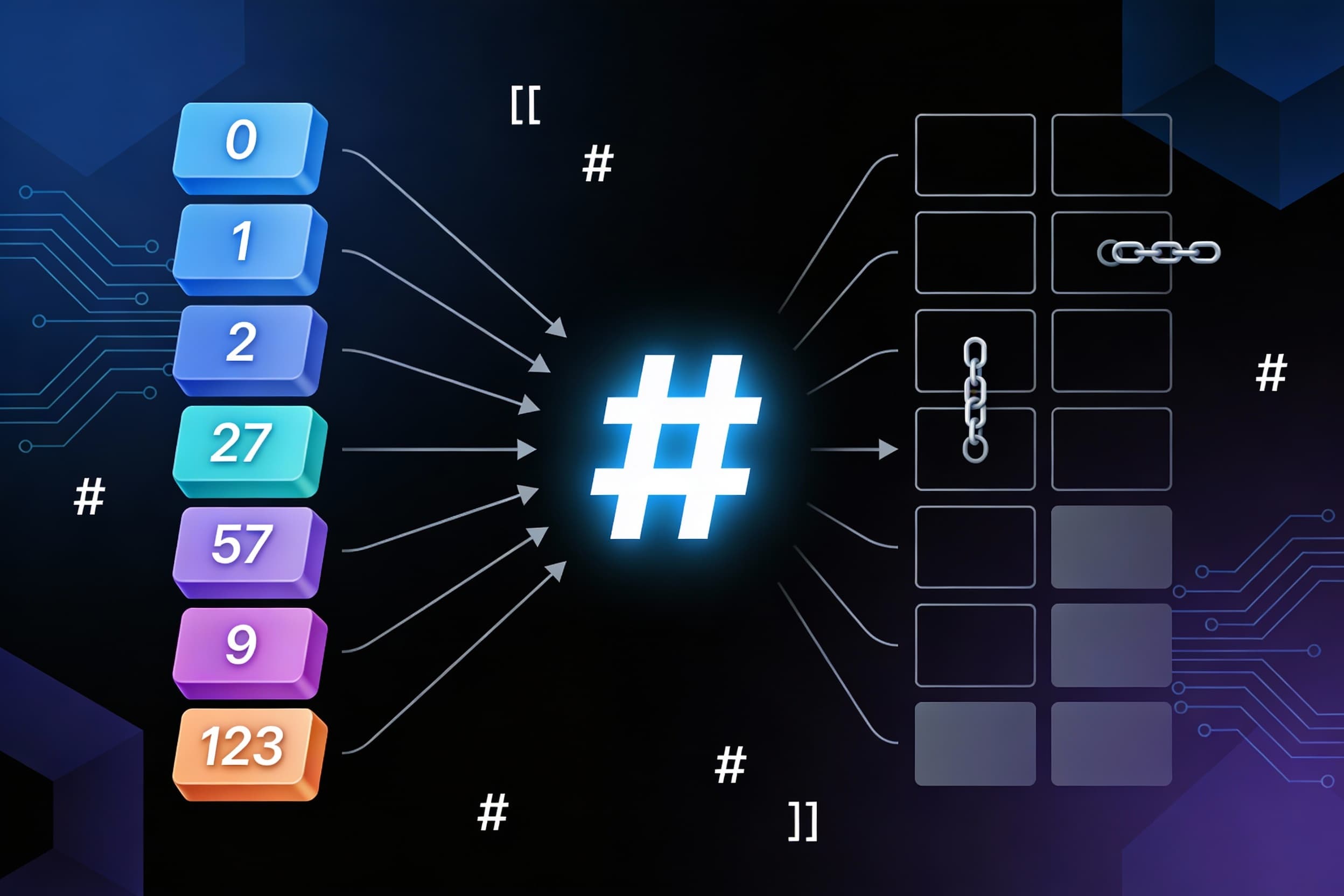
HashMap is a non-linear data structure that lives inside Java's collection framework, alongside other structures like Trees and Graphs (see the generated image above). What makes it special? It uses a clever technique called hashing to store and retrieve data at blazing speeds.

Think of hashing as a smart address system. It converts large keys (like long strings or big numbers) into smaller values that work as array indices. This simple trick transforms your data lookup from slow O(n)O(n) or O(log⁡n)O(logn) operations into lightning-fast O(1)O(1) access times!

Understanding Hashing Mappings

Before diving deeper, let's understand the four types of hashing mappings:

1. One-to-one mapping — Each key maps to exactly one index
2. Many-to-one mapping — Multiple keys can map to the same index
3. One-to-many mapping — One key maps to multiple indices
4. Many-to-many mapping — Multiple keys map to multiple indices

HashMap primarily uses one-to-one and many-to-one mapping strategies to achieve its performance goals.

The Problem: Why Not Just Use Arrays?

Let's say you want to store 7 elements with keys: 1, 5, 23, 57, 234, 678, and 1000.

Using direct indexing (where key = array index), you'd need an array of size 1000 just to store 7 items! That leaves 993 empty slots wasting precious memory. Imagine having a parking lot with 1000 spaces for just 7 cars — totally inefficient!

This is the exact problem hash functions solve.

Hash Functions: The Solution

A hash function takes your key and calculates which array index to use. The beauty? You can now store those same 7 elements in an array of just size 10!

The most common hash function uses the modulus operator:

hash(key)=keymod array sizehash(key)=keymodarray size

Example: With array size = 10:

1. Key 57 → Index: 57mod 10=757mod10=7
2. Key 234 → Index: 234mod 10=4234mod10=4
3. Key 1000 → Index: 1000mod 10=01000mod10=0

Now you only need an array of size 10 instead of 1000. Problem solved!

Three Popular Hash Function Types

Modulus Method

The most widely used technique. Divide the key by array size (or a prime number) and use the remainder as the index.

index=keymod sizeindex=keymodsize

Mid Square Method

Square the key value, then extract the middle digits to form your hash value.

Example: Key = 57 → 572=3249572=3249 → Extract middle digits "24"

Folding Hashing

Divide the key into equal parts, add them together, then apply modulus.

Example: Key = 123456

1. Split into: 12, 34, 56
2. Sum: 12+34+56=10212+34+56=102
3. Apply modulus: 102mod 10=2102mod10=2

The Collision Problem

Here's the catch: sometimes two different keys produce the same index. This is called a collision.

Example:

1. Key 27 → 27mod 10=727mod10=7
2. Key 57 → 57mod 10=757mod10=7

Both keys want index 7! We need smart strategies to handle this.

Collision Resolution: Two Main Techniques

Technique 1: Open Chaining (Separate Chaining)

Mapping Type: Many-to-one

When a collision happens, create a linked list at that index and store all colliding values in sorted order.

Example: Keys 22 and 32 both map to index 2:

Advantage: Simple and works well in practice

Drawback: If too many collisions occur, the linked list becomes long and searching degrades to O(n)O(n). However, Java's collection framework uses highly optimized hash functions that achieve amortized O(1)O(1) time complexity.

Technique 2: Closed Addressing (Open Addressing)

Mapping Type: One-to-many

Instead of creating a list, find another empty slot in the array. There are three approaches:

Linear Probing

When collision occurs, check the next index. If it's occupied, keep checking the next one until you find an empty slot.

Hash Function:

h(x)=xmod sizeh(x)=xmodsize

On Collision:

h(x)=(h(x)+i)mod sizeh(x)=(h(x)+i)modsize

where i=0,1,2,3,…i=0,1,2,3,…

Example: Keys 22 and 32 both map to index 2:

1. Store 22 at index 2
2. Try 32 at index 2 → occupied
3. Check index 3 → empty, store 32 there

Problems:

1. Clustering: Keys bunch together in adjacent indices, slowing down searches
2. Deleted Slot Problem: When you delete a key, it creates an empty slot that breaks the search chain

The Deleted Slot Problem Explained:

1. Keys 22 and 32 are at indices 2 and 3
2. Delete key 22 from index 2
3. Now when searching for key 32, the algorithm reaches index 2 (empty), thinks key 32 doesn't exist, and stops searching!

Solution: Mark deleted slots with a special marker (like -1) or perform rehashing after deletions.

Quadratic Probing

Same concept as linear probing, but instead of checking consecutive slots, jump in quadratic increments: 1, 4, 9, 16, 25...

Hash Function:

h(x)=xmod sizeh(x)=xmodsize

On Collision:

h(x)=(h(x)+i2)mod sizeh(x)=(h(x)+i2)modsize

where i=0,1,2,3,…i=0,1,2,3,…

Advantage: Significantly reduces clustering

Drawback: Still suffers from the deleted slot problem

Double Hashing

The most sophisticated approach! Uses two different hash functions to create unique probe sequences for each key.

First Hash Function:

h1(x)=xmod sizeh1(x)=xmodsize

Second Hash Function:

h2(x)=prime−(xmod prime)h2(x)=prime−(xmodprime)

On Collision:

h(x)=(h1(x)+i×h2(x))mod sizeh(x)=(h1(x)+i×h2(x))modsize

where i=0,1,2,3,…i=0,1,2,3,…

Advantage: Effectively avoids clustering and provides the best performance among probing techniques

Load Factor: The Performance Indicator

The load factor tells you how full your hash table is:

Load Factor=Number of elementsArray sizeLoad Factor=Array sizeNumber of elements

Performance Guidelines

1. Load Factor ≤ 0.5 → Good performance, fast operations
2. Load Factor > 0.7 → Poor performance, time to rehash

Examples

Bad Load Factor:

1. Array size = 10, Elements = 8
2. Load Factor = 8/10=0.88/10=0.8
3. Action: Rehash the array (typically double the size)

Good Load Factor:

1. Array size = 200, Elements = 100
2. Load Factor = 100/200=0.5100/200=0.5
3. Action: No changes needed, performing optimally

What is Rehashing?

When the load factor exceeds the threshold (usually 0.7), the hash table is resized — typically doubled in size. All existing elements are then rehashed and redistributed into the new larger array. This maintains optimal performance as your data grows.

Performance Summary

HashMap delivers exceptional average-case performance:

1. Insertion: O(1)O(1)
2. Deletion: O(1)O(1)
3. Search: O(1)O(1)

However, in the worst case (many collisions with poor hash functions), operations can degrade to O(n)O(n).

The key to maintaining O(1)O(1) performance:

1. Use a good hash function
2. Choose an appropriate collision resolution strategy
3. Monitor and maintain a healthy load factor
4. Rehash when necessary

Conclusion

HashMap is one of the most powerful and frequently used data structures in programming. By understanding hashing techniques, collision resolution strategies, and load factors, you can write more efficient code and make better design decisions.

Whether you're building a cache, implementing a frequency counter, or solving complex algorithm problems, HashMap is your go-to tool for fast data access!